

Introduction
Strategy for a non-linear solution
Rheological study
Friction of Coulomb
Cracks Opening
Model Development
Application
Conclusion
Introduction
Nowadays, the necessity to use perfect seismic evaluation methods for structures subsequent to earthquakes becomes more obvious than ever. Predicting resistance level of an existing RC structure is much more difficult to understand and its behavior is principally unidentified consequential from material nonlinearity. There are possibilities to estimate material nonlinearity’s behavior during and after earthquake by using increasingly powerful physical models and numerical integration procedures.
Transition from conventional computational codes based on empirical design to a more scientific approach requires use of analytical models representative of the complex behavior of reinforced concrete elements subjected to a seismic signal in numerical simulations instead of very expensive real-scale tests. Many analytical and experimental studies underwent deep studies to understand the behavior of RC structures.
Numerical models have been developed to simulate the nonlinear behavior due to the material constituent of RC structures, including the layered fiber model used for a global analysis and the finite element model for a refined analysis.
In a fiber model, each section of the structure is divided into a number of layers or fibers [1] by modeling each layer by a constitutive law appropriate for the material of that particular layer. This modeling has two associate advantages [2]:
- RC section is derived from the uniaxial stress-strain of the fibers and the three-dimensional stress such as the concrete confined by the transverse steel can be incorporated into the uniaxial stress-strain relationship.
- Interaction between the bending moment and the axial force can be described in a rational way.
Fiber modeling is founded on the assumption that plane sections remain plane after deformation, which implies a perfect bond between the longitudinal reinforcements and the surrounding concrete [3], [4].
The evolution of stiffness under macro fiber modeling requires refined rheological models for constitutive laws.
Several hysteresis models were developed in a recent past. They can be largely classified into two types: Polygonal Hysteresis Model (PHM) and Smooth Hysteresis Model (SHM).
Models based on linear behavior by part are PHM’s models. Such models are generally justified by a state of the real behavior of an element or a structure, such as initial or elastic cracking, flow, stiffness degradation and resistance, and closing or opening of cracks. Among several examples, one can quote [5]: The Clough model, Takeda’s model, and the model with three-parameters of Park et al. Sivaselvan and Reinhorn presented in a detailed description, a general framework for PHM’s. On the other hand, the SHM’s models refer to models with a continual change in stiffness leading to yielding, while abrupt changes are due to unloading and deteriorating behavior. The Bouc-Wen models as well as the Ozdemir model are examples of SHM’s.
In structural analysis, material nonlinearity is defined in the level of the cross section [6]. Basically, there are two approaches to represent the constitutive behavior of the section;
-Using direct relation between efforts (such as axial force and bending moments) and the generalized deformations (such as axial deformation and reference curvature).
-Integrating material strain-stress relations defined for material point in the cross-section.
Disadvantage of the first approach requires a specific force-strain relationship for all cross sections. Although, this is not a serious problem in case of standard shapes, the approach is not well adapted to the reinforced concrete reinforcements for all possible variability of sections designs. To explain coupled behavior, this approach is usually based on plasticity theory and uses a function for yielding cross-section in terms of resultants of stress. Another disadvantage of this method is the difficulty in representing the partial yielding in the cross-section.
In the second approach, very accurate constitutive laws are obtained at the expense using a grid refining to evaluate numerical integrals through across sections, while a great number of intake points can be necessary. Besides, computer effort to perform numerical integrations and storage of history variables related to each one of these points is time consuming and the method gets more expensive, especially for complex three dimensional structures with tremendous elements. However, the most important advantage is the ability to handle different types of cross sections, which is particularly convenient in reinforcement’s analysis. In addition, yielding and partial cracking of the cross section can be characterized in a simple and precise way. This approach is particularly advantageous when the uniaxial state of effort at the material point’s cross section is easily made. In this situation, the method is called fiber discretization technique. For this type of stress condition, great precision is achieved, and flexibility is possible in terms of material relationships.
Many work for hardening laws with different loading/unloading criteria, residual or thermal stresses can be easily considered with this approach. For example, representation of RC section (shear), with realistic material models, becomes very simple.
The objective of this research is to develop a rheological model allowing nonlinear numerical simulations of the whole system (embedded material) excited by cyclic loads from an earthquake origin. This procedure requires a calibration dictated by laws of physics.
The framework and hypotheses adopted throughout this modeling analysis are:
-Continuum medium is three-dimensional;
-Transformations are infinitesimal and the assumption of small perturbations is considered;
-All viscous properties are neglected;
-All thermal effects and in general any coupling with other physical phenomena are ignored.
Strategy for a non-linear solution
Nonlinear problems can be solved with an incremental procedure along with an iterative strategy. The incremental procedure will lead to an increasing error. An iterative solution procedure with a specified algorithm must be used to correct these errors. Therefore, the combination of incremental and iterative procedures is used as a basis for a nonlinear analysis. During the analysis, the next predictive step and the stiffness matrix as well as the unbalanced and residual vectors are determined at any iteration. We then, opt for a controlled load iteration strategy using the Newmark method for each incremental load, calculate the incremental moves with the current stiffness and the unbalanced force, and add the total displacements. Each loading step is applied in turn, and iterations are performed for each increment until equilibrium is reached between loadings and internal resistance stresses according to the Newton-Raphson method.
A very small elementary stiffness or a negative elementary stiffness can involve a divergence. To avoid such problems, it is recommended that the individual diagonal elements are not lower than E/1000 in value [7], where E is the elastic modulus of the concrete. Besides, stiffness degradation occurs due to geometric effects and also the elastic stiffness with an increasing ductility. It has been found empirically that the stiffness degradation can be accurately modeled by the pivot rule [5].
Rheological study
Rheological models postulate existence, at the microscopic level, using elementary mechanisms (springs, slides, dashpots...) is associated so that it reproduces the observed behavior. The slide model represents rigid-plastic behavior: there is no deformation (rigid body) as long as the threshold of plasticity is not reached. It is reversible once it holds all the generated deformation. A more realistic behavior for a solid is elastoplastic: the behavior is elastic but an unrecoverable deformation develops if the threshold is reached.
Combining spring and slide in series (see Figure 1a) produces perfect elastoplastic behavior (Saint-Venant or Prandt). Modeled in Figure 1c, the system limited to an absolute value is greater than σy. The model is without work hardening, since the level of stress does not vary any more or goes beyond the elastic range. There is no energy stored during the deformation, and the heat dissipation is equal to the plastic power. The model is able to reach infinite strains under a constant load, leading to the collapse of the system by excessive strain.
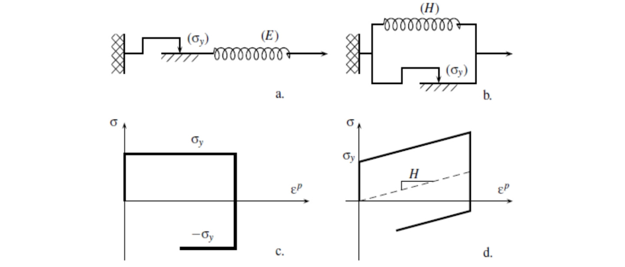
Combinations of spring slide in parallel (Figure 1b) matches the linear kinematic hardening behavior (after Prager) illustrated in Figure 1d. In this case, the hardening is linear [8]. It is known as kinematic because it depends on the actual value of the plastic strain. In this form, the model is rigid-plastic and it becomes elastoplastic if a spring is added in series.
By adding a mass to this model, the system becomes hysteresis. Masing’s model (Figure 2) is a classical hysteresis model connecting an elastic element (Hooke) to a number of plastic elements (Saint-Venant) [9]. This model displays energy dissipation during cycles.
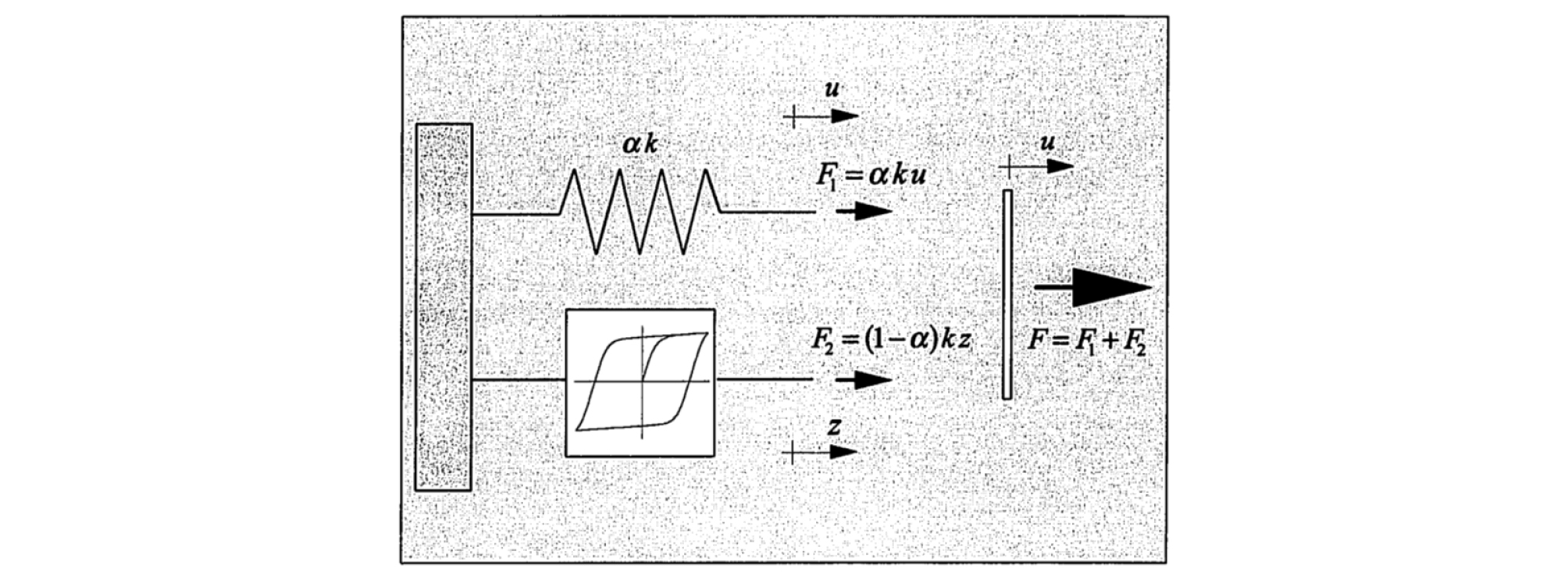
Bouc-Wen model [10], [11] (see Figure 3) is widely used in random vibrations for non-linear hysteresis systems. The differential equation of this model reflects the local history dependence by presenting an additional state variable. Appropriate choice of model parameters can represent a broad variety of behavior such as hardening or softening or near bilinear hysteresis behavior. This model can also be generalized to include hysteresis pinching and stiffness / force degradation [12].
Spacone [1] proposed an extension form to standard Bouc-Wen model (Figure 4) which is modified by presenting the concept of intrinsic time according to endochronic theory. The constitutive differential law is numerically integrated to obtain an incremental moment-curvature relationship. However, parameters choice of the moment-curvature law necessary to adapt a given behavior (obtained from an experimental test) is not simple: the number of parameters to be specified and the corresponding behavior models are very different. Some combinations of parameters lead to non-physical behaviors or inconsistent behavior with the rheological model from which the model is initially derived. It is due to empirical way that the model describes the pinching: on the one hand including the pinching, the range of behaviors that the model can simulate is expanded, but on the other hand it presents non-physical curves. It follows that particular care must be given to the parameters choices [1].
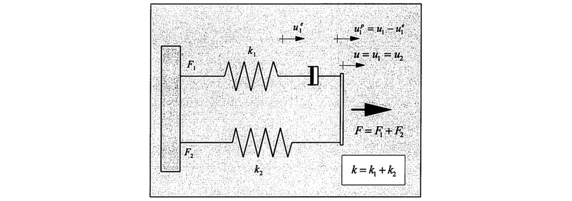
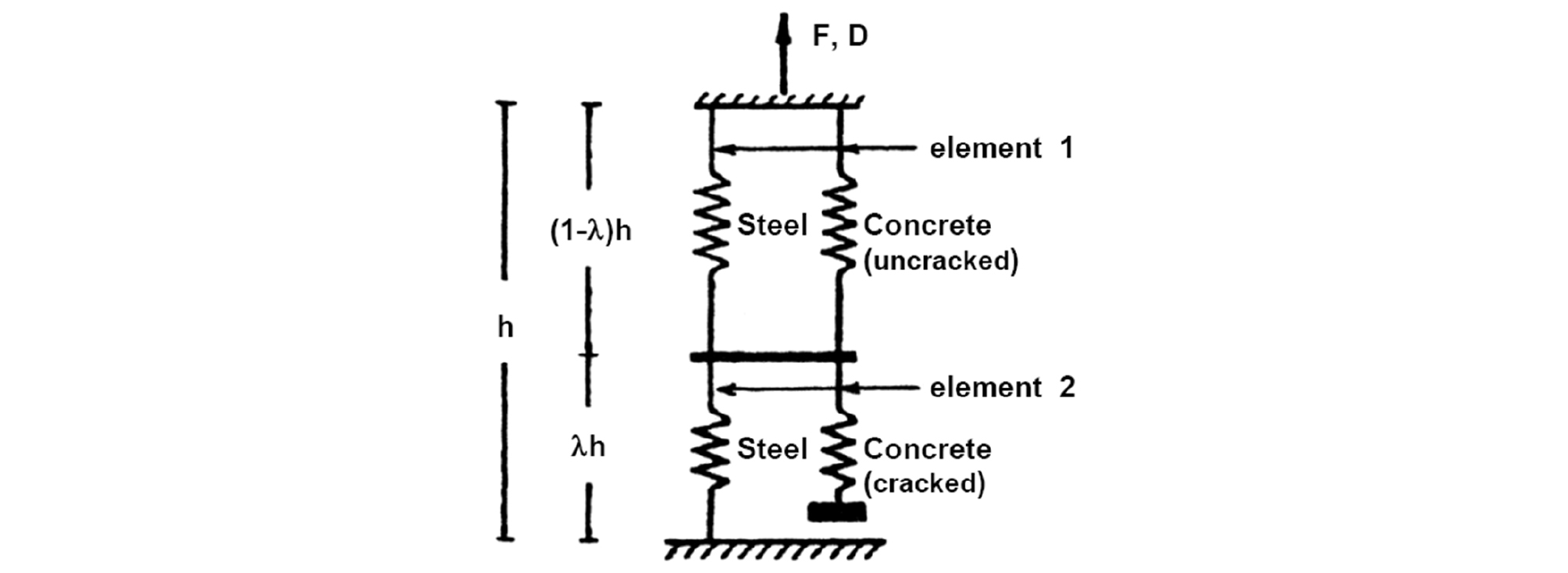
Vulcano and Bertero [13], [14] and [15] propose a hysteresis model to represent RC walls in two axial elements in series as shown in Figure 5. Element 1 in Figure 5 is a one-component model representing the overall axial stiffness of column segments in which the bond is still active, while element 2 is a two-component model representing the axial stiffness of the remaining segments of steel (s) and cracked concrete (c) for which the bond are almost completely deteriorated. This model is intended to idealize the main characteristics of the actual hysteresis behavior of materials and their interaction (yielding and hardening of steel, concrete cracking, contact stresses, bond degradation, etc...).

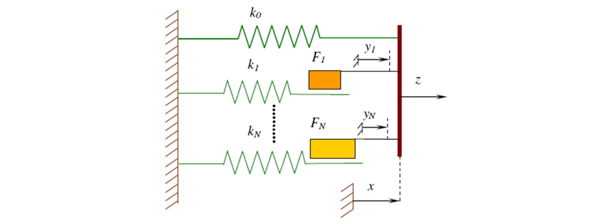
Vulcano, Bertero, and Colotti model [16], [15] with parallel multi-components represents a model with multiple-vertical-line elements (see Figure 6).
This model gives refined description for flexural behavior of the wall by:
- Modifying the geometry of the wall model to gradually account for the progressive yielding of the reinforcement.
- Using more refined hysteresis rules based on the actual behavior of the materials and their interactions to describe the response.
The two elements in series represent the axial stiffness of the column segments in which the bond remained active (element 1) and those segments for which the bond stresses are negligible (element 2). Unlike the original two-element axial series model, element 1 consists of two parallel components to explain the mechanical behavior of uncracked and cracked concrete (c) and reinforcement (s).
An undimensional parameter λ is introduced to define the relative length of the two elements (representing cracked and no cracked concrete) to explain the tensile stiffening.
Friction of Coulomb
Coulomb proposed in 1785, the first friction law, known as Amontons-Coulomb law. This law defines a friction force proportional to the compressive force.
Friction between the grains during an oscillatory movement dissipates energy. Then, Coulomb proposed a force maintaining two surfaces in contact proportional to the applied normal effort (see Figure 7);
| $$\mathrm F=\mu\mathrm N.$$ | (1) |

Friction coefficient (μ) is a dimensionless scalar value describing the relationship of friction force between two bodies and the pressure force maintaining them against each other. Friction coefficient depends on used materials. Friction force is always applied in the opposite direction of the movement (dynamic friction coefficient) or of potential movement (static friction case) between two surfaces. Friction coefficient is an empirical measure, evaluated experimentally. Most of materials, under dry conditions, have coefficient values that range from 0.1 to 0.6. Friction coefficient for concrete/steel pair is 0.45 and for concrete/concrete a coefficient of friction is approximately 0.57.
Cracks Opening
Based on (ACI 224R-90) Committee for beams analysis measurements, factors affecting flexural cracks widths can be;
- Stress or strain in steel is the most significant factor on cracks width.
- Concrete thickness that covers the reinforcement bar and concrete section around each bar are important geometric variables.
- Crack opening in tensile part is affected by the stress gradient of steel tensile part.
- Bars diameter is not considered as important variable.
To explain the main factors affecting crack width, the ACI 224 recommends the crack opening formula in flexion [17], based on Gergely-Lutz equation;
| $${\mathrm W}_{\mathrm c}=2.2\beta\varepsilon_{\mathrm s}\sqrt[3]{{\mathrm d}_{\mathrm c}\mathrm A}$$ | (2) |
Where A is the section area of symmetrical steel RC divided by steel bars number (in inch²) and dc corresponds to the thickness cover from tensile part to the center of the narrowest bar.
Based on a physical model, Frosch [18], [19] developed the following predict crack width equation;
| $${\mathrm W}_{\mathrm c}=2\frac{{\mathrm f}_{\mathrm s}}{{\mathrm E}_{\mathrm s}}\beta\sqrt{\mathrm d_{\mathrm c}^2+(\mathrm s/2)^2}(\mathrm{in}\;\mathrm{inch}\;\mathrm{unit}).$$ | (3) |
Where s is the longitudinal reinforcement bars spacing (in inch), ƒs is steel stress (in ksi) and Es corresponds to the Young’s modulus for steel reinforcements (in ksi unit),
| $$\beta=1+0.08{\mathrm d}_{\mathrm c}$$ | (4) |
In which dc is the coating’s thickness in the tension part along perpendicular axis to the neutral axis (perpendicular distance to the neutral axis between edge of tension part and the nearest reinforcement bar surface center) (in inch unit).
Model Development
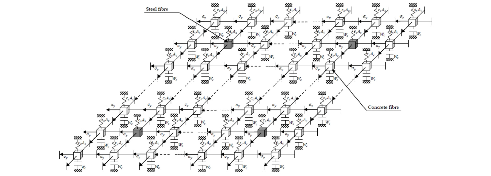
By inspecting the overall macroscopic models mentioned above, the concrete fibers are represented by a rheological model described by a spring with EcAc as stiffness and slide taking into account the Coulomb friction force where the uniaxial stress of the fiber is limited by-σy ≤ σ ≤ σy. In addition, concrete degradation is essentially due to micro-cracks, micro-cavities taking place in the same time of residual strains and stiffness loss [20]. It is assumed that these two phenomena are coupled and the damage makes it possible to describe them [21], [22]. A function wc is integrated to the model representing the opening and closing cracks along the fibers (see Figure 8). The stress is given by [23], [24].
| $$\sigma_{\mathrm c}=\mathrm M\ddot\varepsilon+\mathrm K.(\varepsilon‐\mathrm{sgn}(\dot\varepsilon).{\mathrm w}_{\mathrm c})\leq\mathrm{sgn}(\dot\varepsilon)\mu\mathrm N$$ | (5) |

However, steel fibers are represented by associating a spring EsAs as stiffness and a slider with a Coulomb frictional force, where uniaxial stress of the fiber is limited by -σy≤ σ ≤ +σy (see Figure 8). The stress is written as [23];
| $$\sigma_{\mathrm s}=\mathrm M\ddot\varepsilon+\mathrm K\varepsilon\leq\mathrm{sgn}(\dot\varepsilon)\mu\mathrm N$$ | (6) |
Note that:
Sgn ( ) corresponds to a Signum function, defined as -1.0, 1 for values that are negative and zero for the positive ones.
ε represents a instantaneous strain fiber
represents an instantaneous strain velocity of the fiber
represents an instantaneous strain acceleration of the fiber
M is the mass of the fiber and K is its stiffness.
In this research work, analysis is based on two important principles (Figure 9):
-First, RC element section keeps elastic or more or less elastoplastic state, which avoids the use of failure criterion since the limitation of the macro-fiber model during the evaluation of the severe resistance (softening) and degradation of stiffness during collapse. Yielding fibers are excluded from the strength calculations.
-Second, the structural element stiffness is updated by using numerical integration procedure sustained by iterative process to correct the errors, and rheological models for each fiber type.
Application
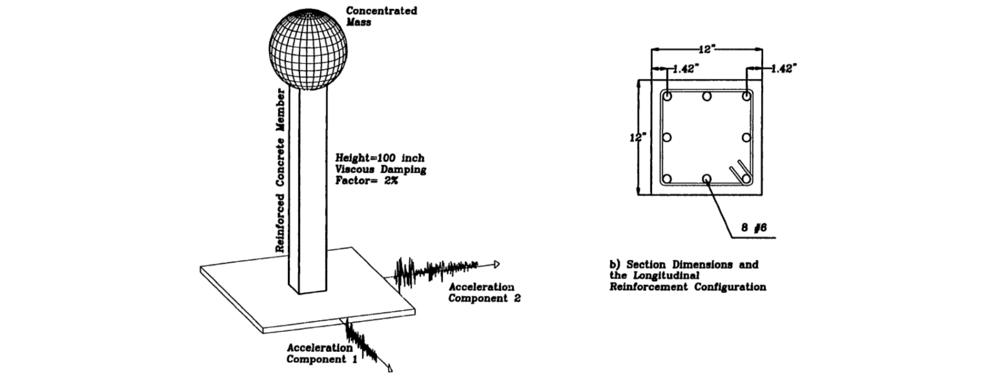
Let’s consider a cantilever material with a density of 2.5t/m3 (see Table 1). Analysis of this material is done using half of its mass concentrated at the top of this cantilever and a viscous damping factor ξ equal to 2% (see Figure 10). For the case of a cantilever embedded at its base and free at its top, the stiffness is given by K = 3E I /L3 and C = 2 ξ as damping.
Table 1. System Characteristics
Biaxial earthquake excitation is taken because considerable strength and energy absorption changes were observed in columns subjected to biaxial loading when compared to those loaded with uniaxial projections of the biaxial deformation paths [4]. In addition, biaxial loading significantly affects nonlinear column behavior comparatively to uniaxial loading [24].
The element is assumed not vulnerable to shear failure, since it is the deformation caused by bending that is greater than that caused by shearing (axial, shear and torsion deformation effects have been neglected [25]). The neutral axis is assumed to be perpendicular to the resulting moments [26].
Response of the cantilever is obtained using the proposed rheological models as constitutive laws relating non-linearity of the material in a bending behavior only. Some arrangements must be done to adapt the calculations to the material complexity such as reinforced concrete.
We are interested in computing the displacement at the tip of the cantilever beam after yielding of the reinforcement at the end section. The algorithm for evaluation of moment for a given curvature is as follows [23], [27];
1 .The section is divided into required a number of fibers in the analysis direction.
2 .For a specific curvature, a location for the neutral axis is guessed and the corresponding axial load is evaluated by integrating the forces of individual fibers in the section.
3 .If the evaluated axial load is equal to the axial load within a predetermined margin, the neutral axis has been found and then the corresponding moment is evaluated and will continue for the next point if any. If the evaluated axial load is not equal to the axial load, the process will be repeated from step 2, and the trial error will continue until the desired level of axial load is achieved.
The algorithm to evaluate the moment curvature results for a specific strain is summarized as follows [23], [27]:
1 .For the required strain (either the concrete strain when positive or steel when negative), select a position for the neutral axis, and the line connecting the point with the required strain and the neutral axis determines the plane for which the axial force should be evaluated.
2 .Evaluate the axial load. If it is equal to the desired level for the step (within the acceptable error margin); the neutral axis is found and the moment will be calculated. Otherwise the process should be repeated for another location of neutral axis, until the proper location is achieved.
The resultant moment on the section may be represented by the two components Mx and My or by a vector M of magnitude and inclined at the angle Ψ=tan-1(Mx/My )to the x axis.
The resultant curvature Φ of magnitude and inclined at the angle θ=tan-1(ΦX/Φy)with respect to the x axis. The moment and curvature vectors nearly coincide in direction throughout the entire range of loading; the maximum difference between the two vectors is of the order of ten degrees [28].
Difference between load angle Ψ and neutral axis angle θ is neglected [29], [30]. Then, the total lateral tip displacement can be written as [31], [27];
| $$\triangle_{\mathrm{to}t}=\triangle_f+\triangle_{\mathrm s}+\triangle_{\mathrm v}$$ | (7) |
Where; Δf is the lateral deflection due to flexure; Δs is the lateral deflection due to reinforcement bond slip; Δv is the lateral deflection due to shear.
The deflection Δf is calculated by summing the static moment of the area under the column theoretical curvature diagram taken about the point of contra flexure. The moment-curvature diagrams were obtained by stress-strain relationships for steel and concrete, respectively
The lateral deflection due to reinforcement bond slip Δs of reinforcing bars is estimated by assuming a constant development length (based on Dragovich experiments [32], 50 times bar diameter for coupled elements and 40 times for uncoupled elements) and a linear decrease of the strain of the bar from the face of the support, up to the end of the defined development length. The slip is calculated for reinforcing bar that has a highest strain in the section.
Calculated slip is converted to rotation using distance between the bar and the neutral axis. Then, deflection of the cantilever free end is calculated by multiplying the rotation due to slip with the length element.
The lateral deflection due to shear Δv is based on linear, uncracked RC element with a maximum calculated contribution of the shear deflection to the total calculated deflection less to 0.35% of the total. The deflection due to the shear at the free end of cantilever for a rectangular section is given by [27];
| $$\triangle_{\mathrm v}=6\mathrm{VL}/5\mathrm{GA}$$ | (8) |
Where;
Δv: shear deflexion.
V: shear force at the tip of cantilever.
G: shear modulus(G=Ec/2(1+ ν))
ν: Poisson ratio supposed to equal to 1/6.
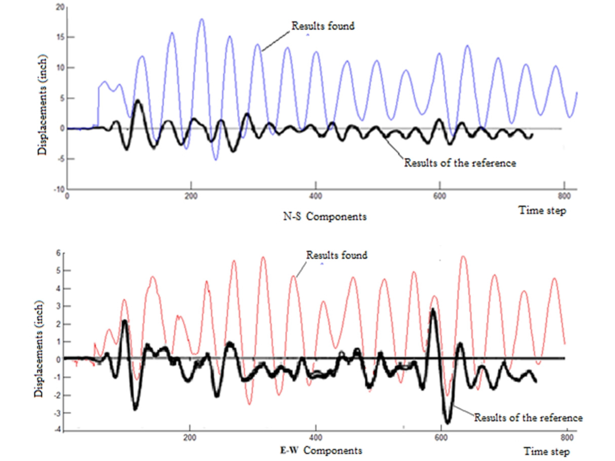
Application of the definitions outlined above is taken to achieved force equilibrium of a reinforced concrete cantilever under a bi-directional signal of EL-CENTRO (California Institute of Technology registration) through a program in a Matlab script show that the displacements at the top are sensitive to the seismic signal since the peaks are recorded during the maximum values of the base acceleration (see Figure 11).
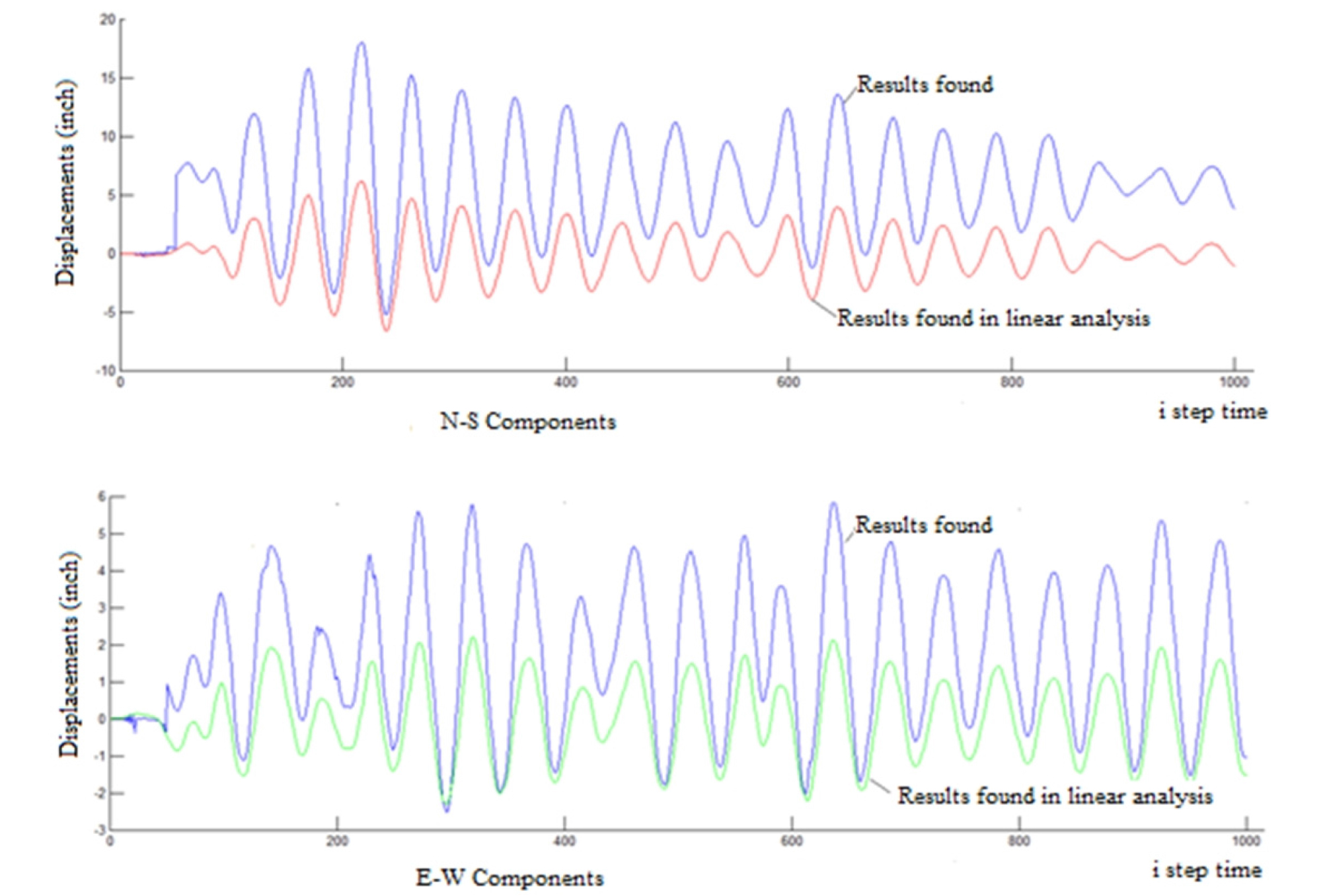
These displacements have similar appearances to those obtained by a linear analysis but with amplification of the order of 3 after the yielding of the current section. In the other hand, divergences occur after a certain number of iterations after the yielding of the section sensitive to the tolerance chosen for the displacement of the top of the cantilever. These divergences make the appreciation of the other parameters (stiffness, moment, damping, stress, acceleration, velocity....) unexpected. The incremental stiffness’s of the cantilever after the first yielding at time t=0.6 sec of the signal increase exponentially up to the order of 10257pound/inch at the end of the process (for initial stiffness Kx = Ky = 26662 pound/inch). In addition, the strains and stresses in the fibers and the incremental moments in the section become extremely excessive.
The results obtained show the aptitude of the proposed model to give heartening results despite the observed discrepancies compared to those given by the reference [27] (see Figure 12), a judicious choice of the resolution strategy and the use of a solver involving methods more adapted to solve the differential equations processed can make the model more reliable.
The numerical difficulty in determining tangent stiffness is frequently found in the following cases:
- In a softening material where the slope stress-strain in loading (increase of the strain) is opposite to the unloading (decrease of the strain) and also the stiffness in one direction can`t follow the incremental strain in the other direction of the incremental stress.
- During an abrupt fall of the strength of a structure or a sudden change in the load transfer mechanism occurs, the loading and unloading (increase and decrease of strain) appears through all the structure.
- During a stress or a strain getting closer to zero.
Conclusion
The basic idea of this research was to develop a model allowing the evaluation of the material stiffness of an RC element of structure after a seismic signal in the time field. After investigation, it turned out that an advanced model requires the use of more sophisticated and optimized numerical processes founded in an object-oriented environment rather than those in an oriented-function environment.
The proposed model introduces the cracking of RC as a cyclic phenomenon incorporated in the behavior of the material itself using empirical formulas adopted by the calculation rules. In addition, the model introduces also internal friction using Coulomb friction which allows excluding the damaged parts of the material in the section.
The stiffness method is useful to get the structure response up to the ultimate resistance stage; but unable to get the behavior of the structure beyond this step. It is also unable to capture the temporary drop in strength due to initial concrete cracking.
This method faces convergence difficulties because the stiffness matrix becomes almost singular at the peak points of the load-displacement curve. Therefore, it is not possible to determine it (sometimes physical or loading conditions dictate the iteration strategy to use); the initial elastic stiffness is therefore used only when the convergence is not completed by tangent stiffness. Once convergence is achieved, the iteration scheme is returned to the tangent stiffness method.
It is proven that there is no preference for controlled load or controlled displacement. The controlled displacement method offers advantages beyond the conventional controlled load method and the proposed model can be coupled with other models capturing different aspects of structural behavior such as geometrical non-linearity or that due to the change of status, soil-structure interaction, and thermodynamic effects.
Our future research will focus in this direction in order to adopt a program that allows the quantification of the desired parameters at any moment of the signal.
