

Introduction
Analytical Method
Overview of the carbonation prediction modeling
Conversion of carbonation velocity coefficient according to experiment environment
Previous linear prediction models
Hamada equation
Kishitani equation
Shirayama equation
Carbonation velocity coefficient prediction using deep learning
Deep learning
Construction method of concrete carbonation coefficient prediction algorithm
Model verification with Experimental Data
Results and Discussion
Carbonation coefficient factor
Results of the DNN model and linear equations using training data
Evaluation of DNN model Based on Experimental Results
Accelerated Carbonation Experiment Results
Results of the DNN model performance using experiment data
Conclusions
Introduction
Reinforced concrete is degraded through contact with external harmful agents in which carbonation is one of the major factors to reduce the durability of the concrete [1]. Concrete carbonation refers to a phenomenon in which the pH of concrete decreases during penetration of carbon dioxide into the exposed concrete, causing corrosion of rebar. Corroded rebar increases in volume, causing cracks in the concrete which reduces the durability of the reinforced concrete [2]. Therefore, it is important to consider the carbonation of concrete owing to carbon dioxide concentration in the atmosphere causes by increasing industrial development and urbanization [3].
Carbonation prediction of the concrete requires considerable changes in the physical and chemical properties and carbon dioxide depending on the actual and experimental conditions. Recently, a method of analyzing and deriving the variables generated during the carbonation of the concrete using machine learning has been proposed. Machine learning is a technique for performing classification or regression on input data. Especially, it can predict the result based on the given data. It has excellent performance in classifying the result through multiple data processing. Already, neural network-based machine learning algorithms have been studied to predict the carbonation of the concrete based on the experimental data [4, 5]. Prediction of carbonation of concrete with the passing of time was studied through the algorithms such as radial basis function network which used the back-propagation network [6, 7], support vector machine using non-probability binary linear classification [8] and decision tree learning which used a decision tree model as a predictive model to go from observations about a target data [9]. Among them, the deep learning algorithm showed better accuracy and shorter analysis than other predictions [10]. In addition, studies have been carried out to analyze the mechanism of carbonation progression of concrete or to use machine learning in the process of carbonation of concrete under the influence of a specific load or temperature [11, 12]. These studies were carried out with machine learning by setting the variable data which are the mixing, curing, and experimental carbonation conditions of concrete and in most cases, using accelerated carbonation experimental data. However, in this study, we predicted the concrete carbonation velocity coefficient after correcting the conditions of carbonation experiment.
In this study, a model-based learning is reviewed that predicts the carbonation coefficient of concrete based on the accelerated carbonation test results of existing studies using deep learning algorithm among neural network-based machine learning algorithms. The DNN model is based on the parameters provided by the deep learning algorithm itself, and the input data are water to binder ratio (W/B), amount of cement, blast furnace slag (BFS), fly ash (FA), coarse aggregate and fine aggregate. The purpose of this study is to investigate the method which is a deep learning-based concrete carbonation prediction and compare the performance with Kishitani, Hamada, and Shirayama equation.
Analytical Method
Overview of the carbonation prediction modeling
The relation of carbonation depth and time has been studied through previous experiments based on Fick's second law, Equation 1 [1, 2].
| $$C=A\sqrt t$$ | (1) |
Where C is the carbonation depth at time t, A is the carbonation velocity coefficient.
The carbonation velocity coefficient A of concrete is the factor that is influenced by type of cement used in concrete, total amount of cement used, water-cement ratio (W/C), type of aggregate, the concentration of carbon dioxide, temperature and humidity of the concrete. Each concrete specimen has different carbonation velocity coefficients depending on the physical and chemical properties of the specimen.
Conversion of carbonation velocity coefficient according to experiment environment
Researchers have considered different environment in which the carbonated concrete experiment was conducted. Before using it for learning, the data was converted to an environment of 5% CO2, 60% relative humidity, and 20°C temperature [13]. Equation 2 can be used to proceed as [14].
| $$A=\cdot\;A_t\;\cdot\;A_{Hu}\;\cdot\;A_{CO_2}$$ | (2) |
Where, , T : temperature, /
19200, Hu : Relative humidity, = (CO2)0.5, CO2 : concentration of carbon dioxide in air
In order to change the environmental condition from the actual environment to standard accelerated carbonation, the difference in the concentration of carbon dioxide should be considered. This can be corrected using Equation 3 [15].
| $$A_{CO_2}=(CO_2/5)^{0.5}$$ | (3) |
Previous linear prediction models
Hamada equation
Hamada's equation suggested the following Equation 4 through test results for 20 years natural exposures [16].
| $$t=\frac{0.003(1.15+3W/C)}{R_a^2{(W/C-0.25)}^2}\;\cdot\;C^2$$ | (4) |
| $$R_a^2=\alpha\;\cdot\;\beta\;\cdot\;\gamma$$ | (5) |
Where, C : Carbonation depth (mm), t : Time (year), W/C : Water to cement ratio, α : coefficient of type of cement (ordinary Portland cement, α=1.0, contain BFS 30 to 40%, α=1.4, BFS over 60%, α=2.2, contain FA 20%, α=1.2), β : coefficient of type of aggregate (natural aggregate, β=1), γ : coefficient according to surface active agent (using air-entertaining agent,γ =0.6, using air-entertaining water reducing admixture,γ =0.4)
Kishitani equation
The Kishitani equation is based Hamada equation, so it is same to Hamada equation when W/C over 60%. It predicts the carbonation depth over the time according to W/C ratio [17].
| $$t=\frac{0.072}{R_a^2(4.6W/C-1.76)^2}\;\cdot\;C^2(W/C\leq0.6)$$ | (6) |
Where, C : Carbonation depth (mm), t : Time (year), W/C : Water to cement ratio
Shirayama equation
Shirayama equation derives carbonation depth considering W/C and Other variables [16].
| $$t=R_b\;\cdot\frac{50}{{(W/C-0.38)}^2}\;\cdot\;C^2$$ | (7) |
| $$R_b\;=\;\alpha\;\cdot\;\beta\;\cdot\;\gamma$$ | (8) |
Where, C : Carbonation depth (mm), t : Time (year), W/C : Water to cement ratio, α : coefficient of type of cement (ordinary Portland cement, α=1.0, up to contain BFS 30%, α=0.4, up to contain BFS 60%, α=0.5, BFS 60% over, α=0.3, contain FA 20%, α=0.3), β : coefficient of type of aggregate (natural aggregate, β=1), γ : coefficient according to surface active agent (using air-entertaining agent, γ=2.8, using air entertaining water reducing admixture, γ=6.2)
Carbonation velocity coefficient prediction using deep learning
Deep learning
Deep learning is one of the machine learning algorithms and uses a variety of nonlinear function algorithms to achieve high accuracy prediction performance. It is also called a deep neural network learning method. The deep learning is composed of an input layer, an output layer, and a hidden layer, and learning is performed at a node inside the hidden layer [18, 19]. DNN model shows accurate predictions. However, if the learning is excessed, DNN model shows accurate predictions only for the data used in the training. This is called overfitting in the deep learning [20, 21, 22]. This is a major factor in lowering the accuracy of the DNN model, so some methods are applied such as dropout and normalization algorithm. Dropout is used to reduce the learning time through the process of determining the importance of weights by randomly deactivating the nodes of the hidden layer. Normalization algorithm is used to reduce weights which is returned to each node.
Construction method of concrete carbonation coefficient prediction algorithm
The data used in the analysis were based on the results of accelerated carbonation experiments in the existing literature, and 291 concrete mix proportions between 30 and 70% of water-binder ratio were used. Factors affecting the analysis were W/B, unit cement content, unit water content, BFS and FA, fine aggregate and coarse aggregate. The data used in the training can be found in appendix A.
Table 1 shows the analysis plan for the predictive model. The DNN model uses error backpropagation as a learning method based on supervised learning, and sets weight change according to the progress of learning by stochastic gradient descent through the activation function [23]. The activation function used the rectified linear unit (ReLU) that showed higher performance in predicting the carbonation velocity coefficient among ReLU and Leaky ReLU, which are mainly used [24]. As an optimizer, we used adaptive moment estimation (ADAM), which has the function of reducing the initial learning rate and reflecting the amount of changes in the previous as learning progresses [25]. Also, to improve the learning speed of the model, Dropout was used for all hidden layers [26] and the ratio of inactive nodes was set to 50%. Since the normalization function of the model is composed of the DNN model based on the gradient descent method. In order to reduce the learning weight effect of the carbonation velocity coefficient, the L2 function is used to reflect the influence of the previous weight on the new weight [27]. The result of learning was confirmed using validation data, and the ratio was set to 15% of the total data. In addition, the learning error used for mean absolute percentage error rate (MAPE). The model with the lowest learning error is compared with the experiment results.
Table 1. Composition of model
| Analysis Factor | Analysis parameter |
| Hidden Layer | 5 |
| Batch Size | 64 |
| Activation Function | ReLU |
| Dropout | 50% |
| Regularization Algorithm | L2 |
| Validation Data Ratio (%) | 15 |
Model verification with Experimental Data
In this study, the error rate of carbonation coefficient was confirmed by applying part of the data as validation data. The error rates between the previous experimental value and the prediction value of the model-based learning using 50 data were compared. Then, it was evaluated using the linear prediction equation. The linear carbonation equation is a regression equation produced through the experiment, and the carbonation velocity coefficient according to the carbonation influencing factor to predict the carbonation depth over time using the experimental result. In this study, the linear prediction equations are derived from predictions using the Kishitani, Hamada, and Shirayama equation.
Table 2 shows the mix proportion of concrete specimens used in concrete for accelerated carbonation experiments conducted to determine the accuracy of the DNN model.
Table 2. Mix proportions of concrete for accelerated carbonation test
The mixing level was considered for W/B and BFS substitution. The carbonation velocity coefficient of test specimens were calculated from the results of accelerated carbonation test during 1, 4 and 8 weeks. The concrete carbonation velocity coefficients were compared with the carbonation velocity coefficients predicted using the DNN model and the linear carbonation prediction i.e. Kishitani, Shirayama, Hamada equations.
Results and Discussion
Carbonation coefficient factor
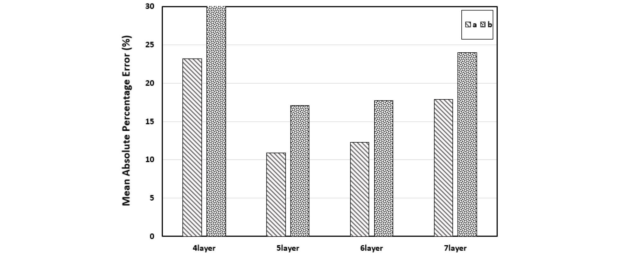
The results of each model are shown in Figure 1. We decided to use 5 hidden layers’ model which 4 to 4 hidden layer shows the best performance between the models where ‘a’ represents a learning rate of 0.0001 and ‘b’ represents a learning rate of 0.00005. Figure 1 shows the MAPE models which are 23.21% in 4l_a, 43.75% in 4l_b, 10.92% in 5l_a, 17.14% in 5l_b, 12.25% in 6l_a, 17.77% in 6l _b, 17.94% in 7l _a, 23.98% in 7l _b.
Results of the DNN model and linear equations using training data
Figure 2 shows the results of carbonation velocity coefficient for 50 specimens and the DNN model results are compared with other models. The carbonation velocity coefficient used for the training is expressed in AT, AK, AS and AH for Kishitani , Shirayama , and Hamada equation, respectively. On the other hand, DNN model used AD as the carbonation velocity coefficient.
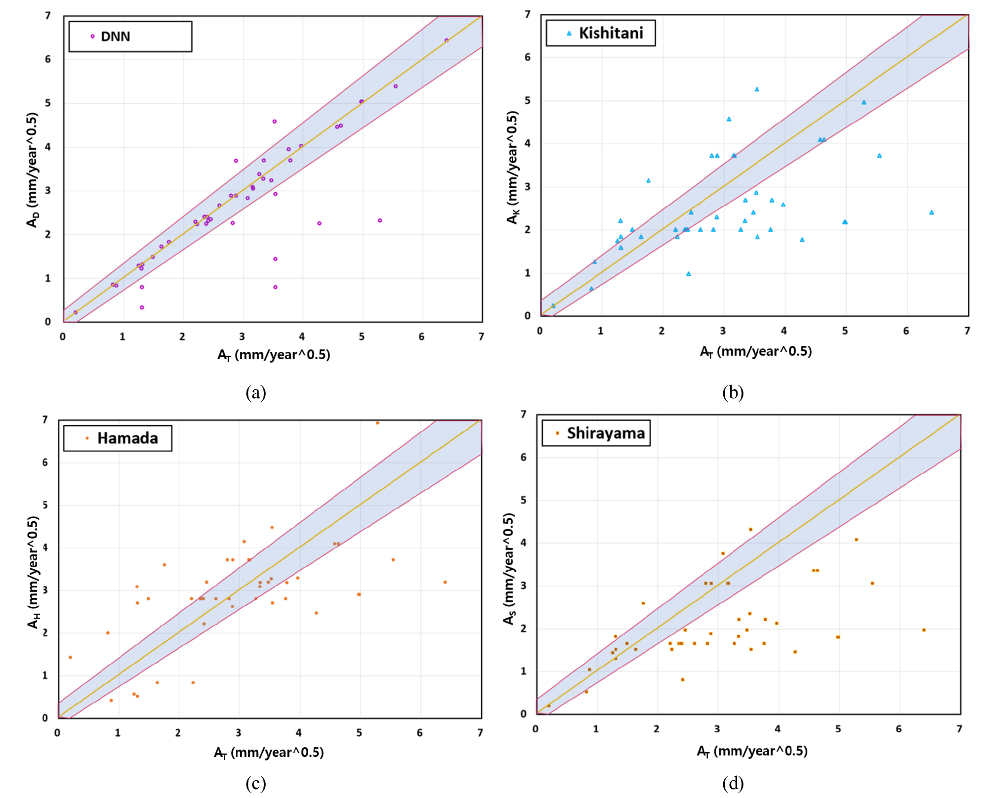
The MAPE result in DNN model shows 9.91%. In the case of linear prediction equation, it shows 31.68%, 49.33% and 43.96% for Kishitani, Hamada, and Shirayama, respectively. It is confirmed that the DNN model error rate is lesser than the linear carbonation prediction equation for the training data results.
Evaluation of DNN model Based on Experimental Results
Accelerated Carbonation Experiment Results
The carbonation depth measurement results are shown Figure 3. From this figure it is found that carbonation depth is increased with increase in proportion of binder as curing duration extended.
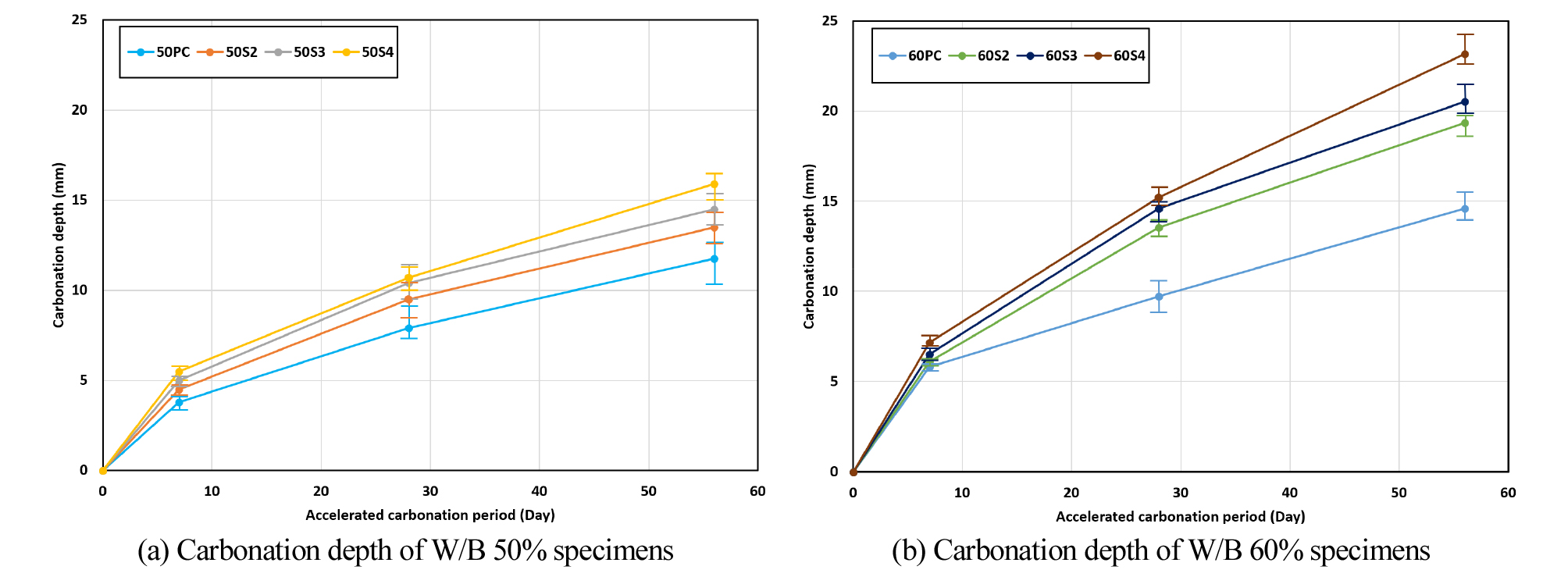
Table 3 shows the carbonation velocity coefficients under the general atmospheric conditions. The carbonation depths from 1, 4, and 8 weeks of 5% CO2 carbonated concrete was converted to carbonation velocity coefficients using Equation 3 i.e. 0.03% CO2. Therefore, the carbonation velocity coefficient is found that as W/B ratio increased, the value increased gradually.
Table 3. Carbonation velocity coefficient of result of the accelerated carbonation test specimens
| Specimen | Carbonation velocity coefficient () |
| 50PC | 2.18 |
| 50B2 | 2.66 |
| 50B3 | 2.87 |
| 50B4 | 2.95 |
| 60PC | 2.79 |
| 60B2 | 3.78 |
| 60B3 | 4.07 |
| 60B4 | 4.26 |
Results of the DNN model performance using experiment data
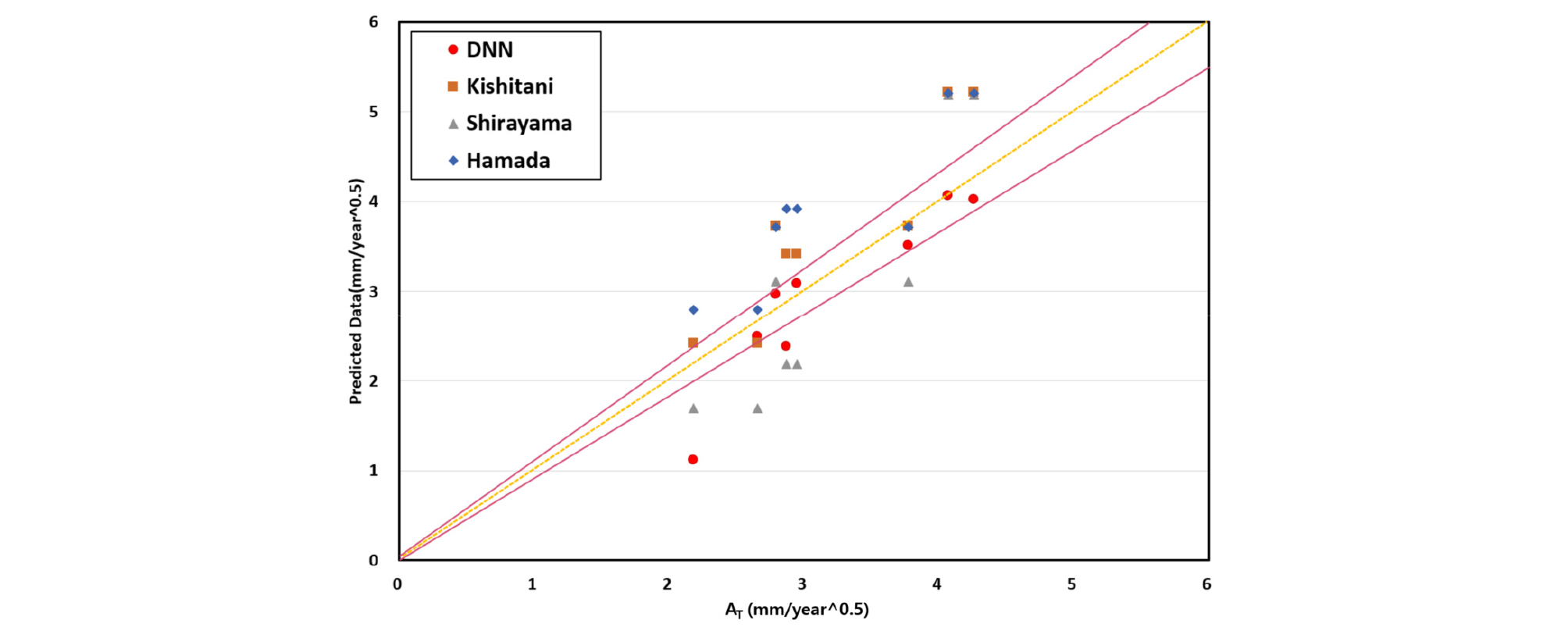
Figure 4 shows the comparison between the predicted data of the DNN model and the accelerated carbonation experimental data. The carbonation velocity coefficient used for present study is expressed in AT. Six data fall within the 10% margin of error and MAPE of DNN model is 12.00%. The error rate of 50PC is found to be 48% owing to the lack of training data in the current category. The mean absolute error between the experimental and predictive equations was obtained to be 29.23%, 18.63% and 30.26% for Kishitani, Shirayama, and Hamada, respectively.
Conclusions
In this study, a model was constructed using DNN for concrete carbonation velocity coefficient and the best was chosen. The error of the experimental and predicted data was confirmed by MAPE. The conclusions of the present can be drawn as follows.
1)In validation test, MAPE was 9.91% in DNN model and it showed the better performance than the linear carbonation prediction equations.
2)The carbonation velocity coefficients () of the specimens was found to be increased as W/B ratio increased.
3)DNN model shows that experimental data fall within the 10% margin error with an average 12.00% absolute error. The error rate of 50PC is found to be 48% owing to the lack of training data in the current category.
4)Compared the MAPE result using Kishitani, Shirayama, and Hamada equations, the prediction performance of DNN model is higher than that of linear prediction model.
